Pile Group Tutorial – Example 3: Pile Group in Sand for TBM Launching

16 hours ago
12 min read

In this tutorial example, the use of the PileGroup program is demonstrated for analysing a pile group subject to TBM launching loading. This example involves a pile group consisting of 20 numbers of 1200 mm diameter CFA piles of 20 m long, which were spaced at three pile diameters in both directions.

Objectives:

Create pile group analysis with linear analysis module
Define linear analysis inputs
Define multiple pile cap loads at different locations
Define multiple load combinations
View pile head results

1.0 Starting a new project after saving and closing the exiting project

1) Start a new project by clicking the New button in the top toolbar or clicking the New submenu under the File main menu.

A confirmation window pops up as shown in the figure below for users to save or abandon the current file before opening the default new file.

Figure 3-1 Start a new project — **Figure 3-1** Start a new project

2) Click Yes button to save the changes to the current input file and open a new default input file for this example.

A default pile group analysis project with 4 piles will be created as shown in the figure below and the users can start creating the pile group analysis inputs by changing the basic parameters.

PileGroup program main input window for pile group analysis inputs — **Figure 3-2** Main input window

3) Save the project

Upon creating a new project in Step 2, the program does not automatically generate a project file name. It is advisable for users to save the project using a file name of their own choosing before they continue further.

2.0 Creating pile group analysis with linear analysis module

By default, nonlinear analysis module based on P-Y, T-Z, and Q-Z curves is used to model soil-structure interaction under lateral and axial loading. To undertake pile group analysis with linear analysis module based on Randolph’s elastic solutions for single piles in homogeneous or Gibson-type soils, follow the steps below:

Open the Analysis Option window by clicking the Define Analysis Option button in the top toolbar or clicking the Analysis Option submenu under the Define main menu.

The figure below shows the Analysis Option-window. By default, the analysis mode is “Nonlinear Analysis Module”. The Pile Installation Type and Settlement Analysis Option inputs will be greyed out, as they do not apply to the linear analysis module

Figure 3-3 Analysis option input window — **Figure 3-3** Analysis option input window

Select “Linear Analysis Module” from the dropdown menu under Analysis Mode input field.
Click OK button to save the inputs and close the input window.

3.0 Defining linear analysis inputs

To create the linear analysis input parameters, follow the steps below:

Open the Linear Analysis Inputs window by clicking the Define Linear Analysis Inputs button in the top toolbar or clicking the Linear Analysis Inputs submenu under the Define main menu.

The figure below shows the Linear Analysis Inputs-window. The three tab menus are “Axial Stiffness”, “Lateral Stiffness”, and “Free Length”.

Figure 3-4 Linear analysis inputs window — **Figure 3-4** Linear analysis inputs window

Select “Using Young’s Modulus (E) and Poisson’s Ratio” from the dropdown menu under Analysis Mode input field.
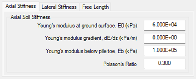
Enter 6 x 10⁴ for Young’s modulus at ground surface, E0 (kPa) under Axial Stiffness sub menu.
Enter 0.0 for Young’s modulus gradient, dE/dz (kPa/m) under Axial Stiffness sub menu.
Enter 1 x 10⁴ for Young’s modulus below pile toe, Eb (kPa) under Axial Stiffness sub menu.
Enter 0.3 for Poisson’s Ratio under Axial Stiffness sub menu.
The final inputs under Axial Stiffness sub menu are shown in the figure below.

Figure 3-5 Axial stiffness input — **Figure 3-5** Axial stiffness input

Enter 6 x 10⁴ for Young’s modulus at ground surface, E0 (kPa) under Lateral Stiffness sub menu.
Enter 0.0 for Young’s modulus gradient, dE/dz (kPa/m) under Lateral Stiffness sub menu.
Enter 0.3 for Poisson’s Ratio under Lateral Stiffness sub menu.
The final inputs under Lateral Stiffness sub menu are shown in the figure below.

Figure 3-6 Lateral stiffness input — **Figure 3-6** Lateral stiffness input

Enter 0.0 for Pile free length above the ground surface (m) under Free Length sub menu.
The final inputs under Lateral Stiffness sub menu are shown in the figure below.

Figure 3-7 Free length input — **Figure 3-7** Free length input

Click OK button to save the inputs and close the input window.

4.0 Creating the pile section

Pile sections must be created before entering detailed inputs like positions and lengths for the pile group. To create a pile section, follow these steps:

Open the Define Section window by clicking the Define Section button in the top toolbar while select the pile section from the list box under Pile Section Sub-window on the left side of the main input window or clicking the Edit button on the right side of the Pile Section Sub-window.
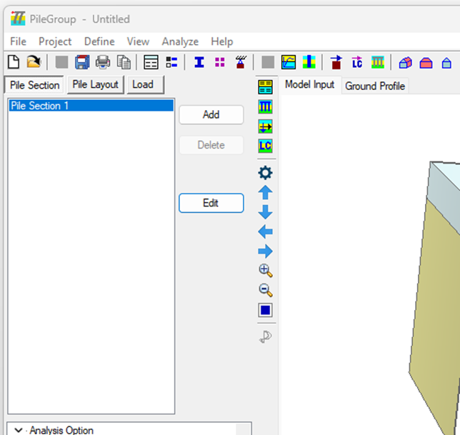
The figure below shows the pile section sub-window on the left side of the main input window. By default, there is one existing pile section with the name of “Pile Section 1”. This existing pile section can be modified by the users.

Pile section inputs for pile group analysis using PileGroup program — **Figure 3-8** Pile section sub-window

The Define Section window pops up as shown in the figure below.
Select “Circular” from the dropdown menu under Section Type.
Enter 1.2 m for Diameter, D under Section Dimension.
Enter 32.8 GPa for Young’s Modulus, E and 0.2 for Poisson’s Ratio, ν under Material Properties.
Enter “Pile Section 1” under Pile Section Name.
Click OK button to save the inputs and close the input window.

Figure 3-9 Section parameter input window — **Figure 3-9** Section parameter input window

5.0 Creating the piles within the pile group using pile layout wizard tool

To create the piles within the pile group, follow these steps:

Open the Pile Group – Layout Table Input window by clicking the Define Pile Length and Layout button in the top toolbar or clicking the Pile Length and Layout submenu under the Define main menu.
By default, there are 4 existing piles pre-defined in the group. Those existing piles can be deleted or modified to suit the actual analysis case. Note that the minimum number of piles with the group is 2. This means that the number of piles cannot be reduced to a number less than 2.
For this tutorial example, there are 6 piles within the group with two battered piles.
Click Add button at the bottom of the window to add one pile into the group. A new pile (5^th pile) with the default position and length will be added to the group. The total number of piles is 5 after this.
Keep clicking the Add button until the total number of the piles is 20. The default input values will be automatically assigned to each newly created pile.
Enter the proper values in the layout input table for each pile. Those values include X Position (m), Z Position (m) and Pile Length (m) for all the piles.
The pile length and layout input window with all the inputs above is shown in the figure below.

Figure 3-10 Pie length and layout input window — **Figure 3-10** Pie length and layout input window

Click OK button to save the inputs and close the input window.
A three-dimensional view for the whole pile group is updated in the Model Input window as shown in the figure below.

Figure 3-11 Three-dimensional view of pile group — **Figure 3-11** Three-dimensional view of pile group

6.0 Defining pile cap connection conditions

To define or modify the pile cap connection conditions, follow these steps:

Open the Pile to Cap Connection window by clicking the Define Pile to Cap Connection button in the top toolbar or click the Pile to Cap Connection submenu under the Define main menu.
The Pile to Cap Connection input window pops up as shown in the figure below.

Figure 3-12 Pile to cap connection — **Figure 3-12** Pile to cap connection

Click Set All to Rigid button at the bottom left of the input window to set the rigid pile head connection for all the piles within the group.
Click OK button to save the inputs and close the input window.

7.0 Creating the loads on the pile cap

To create the loads on the pile cap, follow these steps:

Click the Load button in the tabbed window panel located under the top toolbar on the left side of the main input window to open the Load tab.
By default, the first load case will be automatically selected
Click the Edit button on the right side of the tab window to open the Pile Cap Loads window.
The Pile Cap Loads window pops up and is shown in the figure below.

Figure 3-13 Pile cap load input window
Alternatively, open the Pile Cap Loads window by clicking the Define Pile Cap Loads button in the top toolbar or clicking the Pile Cap Loads submenu under the Define main menu. This will open the Pile Cap Loads window corresponding to the selected load case from the Load tab window.
Change the default Pile Cap Load Name to “Point Load 1”.
Enter -4000 for Axial Load, Fy (kN).
Enter -7500 for Shear Load, Fx (kN).
Enter -3.6 for X Coord (m).
Enter -4.7 for Z Coord (m).
Enter 0 for the other input fields.
Click OK button to save the inputs and close the input window for this load case.
The pile cap load input window for “Point Load 1” is shown in the figure below.

Figure 3-14 Pile cap load input for point load 1 — **Figure 3-14** Pile cap load input for point load 1

Click the Add button on the right side of the tab window to add the second load case.
The Pile Cap Loads window opens with the default inputs and is ready for entry of the second load case.
Change the default Pile Cap Load Name to “Point Load 2”.
Enter -4000 for Axial Load, Fy (kN).
Enter -7500 for Shear Load, Fx (kN).
Enter -3.6 for X Coord (m).
Enter 4.7 for Z Coord (m).
Enter 0 for the other input fields.
Click OK button to save the inputs and close the input window for this load case.
The pile cap load input window for “Point Load 2” is shown in the figure below.

Figure 3-15 Pile cap load input for point load 2 — **Figure 3-15** Pile cap load input for point load 2

Click the Add button on the right side of the tab window to add the third load case.
The Pile Cap Loads window opens with the default inputs and is ready for entry of the third load case.
Change the default Pile Cap Load Name to “Point Load 3”.
Enter 4000 for Axial Load, Fy (kN).
Enter -400 for Shear Load, Fx (kN).
Enter 2000 for Bending, Mz (kN.m).
Enter 10.8 for X Coord (m).
Enter -4.7 for Z Coord (m).
Enter 0 for the other input fields.
Click OK button to save the inputs and close the input window for this load case.
The pile cap load input window for “Point Load 3” is shown in the figure below.

Figure 3-16 Pile cap load input for point load 3 — **Figure 3-16** Pile cap load input for point load 3

Click the Add button on the right side of the tab window to add the fourth load case.
The Pile Cap Loads window opens with the default inputs and is ready for entry of the fourth load case.
Change the default Pile Cap Load Name to “Point Load 4”.
Enter 4000 for Axial Load, Fy (kN).
Enter -400 for Shear Load, Fx (kN).
Enter 2000 for Bending, Mz (kN.m).
Enter 10.8 for X Coord (m).
Enter 4.7 for Z Coord (m).
Enter 0 for the other input fields.
Click OK button to save the inputs and close the input window for this load case.
The pile cap load input window for “Point Load 4” is shown in the figure below.

Figure 3-17 Pile cap load input for point load 4 — **Figure 3-17** Pile cap load input for point load 4

Click the Add button on the right side of the tab window to add the fifth load case.
The Pile Cap Loads window opens with the default inputs and is ready for entry of the fifth load case.
Change the default Pile Cap Load Name to “Resultant Load at the Origin”.
Enter -15800 for Shear Load, Fx (kN).
Enter 1.192 x 10⁵ for Bending, Mz (kN.m).
Enter 0.0 for X Coord (m).
Enter 0.0 for Z Coord (m).
Enter 0 for the other input fields.
Click OK button to save the inputs and close the input window for this load case.
The pile cap load input window for “Resultant Load at the Origin” is shown in the figure below.

Figure 3-18 Pile cap load input for resultant load at the origin — **Figure 3-18** Pile cap load input for resultant load at the origin

8.0 Creating the load combinations

All the analyses in the PileGroup program are carried out using the load combinations which are based on the input pile cap loads. To create the load combinations on the pile cap, follow these steps:

Open the Load Combination window by clicking the Define Load Combination button in the top toolbar or clicking the Load Combination submenu under the Define main menu.

The Load Combination window pops up and is shown in the figure below.

Figure 3-19 Load combination input window — **Figure 3-19** Load combination input window

Enter “SLS Load Case 1” under the column of Name for the first load combination (row).
Enter 1 under the column of Cyclic Load Number for the first load combination.
Enter 1.0 under the column of “Point Load 1” for the first load combination.
Enter 1.0 under the column of “Point Load 2” for the first load combination.
Enter 1.0 under the column of “Point Load 3” for the first load combination.
Enter 1.0 under the column of “Point Load 4” for the first load combination.
Enter 0.0 under the column of “Resultant Load at the Origin” for the first load combination.
Click Add button to create the second load combination.
Enter “ULS Load Case 1” under the column of Name for the second load combination (row).
Enter 1 under the column of Cyclic Load Number for the second load combination.
Enter 1.4 under the column of “Point Load 1” for the second load combination.
Enter 1.4 under the column of “Point Load 2” for the second load combination.
Enter 1.4 under the column of “Point Load 3” for the second load combination.
Enter 1.4 under the column of “Point Load 4” for the second load combination.
Enter 0.0 under the column of “Resultant Load at the Origin” for the second load combination.
Click Add button to create the third load combination.
Enter “SLS Load Case 2” under the column of Name for the third load combination (row).
Enter 1 under the column of Cyclic Load Number for the third load combination.
Enter 0.0 under the column of “Point Load 1” for the third load combination.
Enter 0.0 under the column of “Point Load 2” for the third load combination.
Enter 0.0 under the column of “Point Load 3” for the third load combination.
Enter 0.0 under the column of “Point Load 4” for the third load combination.
Enter 1.0 under the column of “Resultant Load at the Origin” for the third load combination.
Click Add button to create the fourth load combination.
Enter “ULS Load Case 2” under the column of Name for the fourth load combination (row).
Enter 1 under the column of Cyclic Load Number for the fourth load combination.
Enter 0.0 under the column of “Point Load 1” for the fourth load combination.
Enter 0.0 under the column of “Point Load 2” for the fourth load combination.
Enter 0.0 under the column of “Point Load 3” for the fourth load combination.
Enter 0.0 under the column of “Point Load 4” for the fourth load combination.
Enter 1.4 under the column of “Resultant Load at the Origin” for the fourth load combination.
Click OK button to save the inputs and close the input window.
The load combination input window with all the inputs above is shown in the figure below.

Figure 3-20 Load combination input window — **Figure 3-20** Load combination input window

9.0 Define pile group effect

For the linear elastic module, pile group effects are automatically considered by the program and therefore do not require user input. More details for this can be found from the user manual of the PileGroup program.

10.0 Run the pile group analysis

To run the pile group analysis, follow these steps:

Open the Run Analysis window by clicking the Run Analysis button in the top toolbar or clicking the Run Analysis submenu under the Analyze main menu.

Figure 3-21 PileGroup solver window
Click OK button to close the PileGroup Solver window and open the PileGroup Output window to view the analysis results.

Figure 3-22 PileGroup output window — **Figure 3-22** PileGroup output window

For the linear analysis module, the distributed results along the pile length are limited to deflections, bending moments, and shear forces. It is noted that these distributed results are approximate, as only the pile head solutions are exact.

11.0 View pile head results

To check the pile head results from the PileGroup Output window as shown in the figure above, follow these steps:

Open the Pile Head Results window by clicking the Pile Head Results button in the top toolbar or clicking the Pile Head Results submenu under the More Results main menu.
A Pile Head Results window pops up as shown in the figure below. The default pile head result type is Axial Force F2, which shows the axial forces at the pile heads for all the piles within the group. The default load combination selection is the first load combination – “SLS Load Case 1”.

Figure 3-23 Pile head results window for axial force — **Figure 3-23** Pile head results window for axial force

Select Bending Moment, M3 (kN.m) option from the dropdown menu under Pile head result type.
The Pile Head Results window will be updated to show the Bending Moment, M3 results for all the pile heads within the group, as shown in the figure below.

Figure 3-24 Pile head results window for moment M3 — **Figure 3-24** Pile head results window for moment M3

Click the View Output File button to show the tabulated results at the pile heads.
The Tabulated Results at the Pile Heads window opens as shown in the figure below. The tabulated results can be either saved into CSV file by clicking the Save to CSV File button or printed by clicking Print button.